Etiq AI Blog

A Practical Guide to Causal Dataset Repairs

Dr. Laura Hattam

Summary

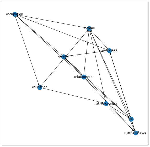
Causal graphs are visual representations of the relationships within a dataset. They are popular due to being easily interpreted by technology and business teams alike. A graph such as the one below, which was constructed (relatively quickly!) using an income dataset, indicates that not only the featuregender on its own influences someone’s income (a direct form of discrimination), but also that genderhas an effect upon someone’s relationship status, which then influences their income (an indirect form of discrimination). Therefore, the feature relationship status should be handled with caution. Beyond these types of observations, there are complex techniques that use the information represented by the causal graphs to mitigate bias. Because of this, causality, and causal repair methods, have emerged as a clear area of interest of ours. However, their implementation is often not straightforward and they can require a relatively high level of user involvement. In this article, we give a detailed account of how one can perform bias identification and mitigation with a causal approach, as well as some pitfalls and difficulties we have encountered.

Introduction

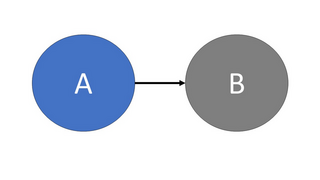
Causality is the study of how certain things, such as events or processes, relate to one another in terms of cause and effect e.g. Event A causes the occurrence of Event B. More recently, this topic has been applied in machine learning to help understand the complex relationships between the different features and outcomes within a dataset. Usually this is with a casual graph, which is a directed acyclic graph (DAG), where the various features/attributes and the decision variable are represented by nodes, and the relationships are depicted by arrows. A simple example of a causal graph, with only two nodes, is depicted in Figure 1, which portrays feature A (node A) having a causal effect upon feature B (node B). To relate this figure to the example given in the summary above, node A would correspond to gender, whilst node B would correspond to income.

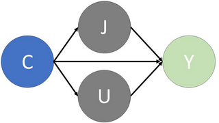
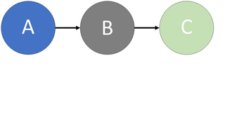
Using a causal graph, causal paths can be highlighted that represent bias within the dataset. In particular, the paths that run from the sensitive attribute node, such as gender or race (demographics vulnerable to discrimination), to the the decision node, indicate bias experienced by the sensitive group. For the path that goes directly from the sensitive attribute to the outcome variable, this represents direct discrimination. Conversely, for the remaining paths that also pass through an ‘unjustified’ attribute (variables that should not be used for decision making), these correspond to indirect discrimination. Once these paths have been identified, certain techniques can be applied to the dataset so that they are modified. These changes aim to eliminate the direct/indirect links between the decision node and the sensitive attribute, and thus, the bias associated with this protected group is removed. In Figure 2, an example of the removal of direct and indirect causal paths is given, which corresponds to the elimination of the discrimination experienced by the sensitive attribute, which could be, say, gender or race.

Repair methods that use a causal approach have been shown to be effective debiasing tools. However, there are some challenges in this area, which include the need for information on the causal structure of the data, such as generating a causal graph, before a debiasing method can be applied. Also, causal repair methods can be difficult to apply in practice. Here, we explore this further by implementing a causal repair algorithm from the literature. Firstly, a casual graph must be constructed, so we detail the different techniques used to perform this, as well as the various publicly available toolboxes related to causal discovery (methods to determine the causal structure of the data). Next, some causal debiasing methods from the literature are discussed in detail, with one implemented in Jupyter Notebook, where a link to the notebook is provided. This is to demonstrate that approaches of this type can potentially be quite involved, including the amount of background work they require. Hence, the overall aim of this article is to provide a practical guide for practitioners that wish to delve into causal dataset repairs.

Causal Discovery

This section discusses the various techniques used for causal discovery, focussing on causal graphs. We believe this is an important area of discussion since it is often necessary to build a causal graph from the data first, before any debiasing (from a causality perspective) can be performed. For further details, refer to Glymour et al. (2019), which provides a good summary of different causal discovery methods.

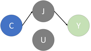
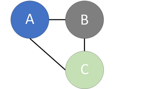
For a constraint-based approach, in order to identify the causal relationships within a graph, the conditional independence relationships in the data must be established, which basically define if certain features are independent of other features, which might be conditional upon another set of features. To outline these relations, it generally requires undertaking statistical tests on the data using such techniques as the Chi-Square test of conditional independence, or the more complex kernel-based conditional independence test (see Zhang et al. (2011)). Then, such methods as the Peter and Clark (PC) algorithm (see Spirtes et al. (2001)) are applied to build the casual graph. This entails starting with all the nodes connected in an undirected graph, then the edges are removed systematically and arrows are introduced according to the conditional independence relations. A simple example of the PC algorithm is given in Figure 3, which starts, on the left, with the three nodes A, B and C all linked with undirected edges. Then by imposing the relation A is independent of C, given B (AꓕC|B), through a series of steps, which includes removing the edge from A to C as they are independent and introducing arrows to represent that C is conditional upon B, the causal graph on the right is formed. There are many variations on the PC method such as the Really Fast Causal Inference (RFCI) algorithm (see Colombo et al. (2012)), which, as the name suggests, attempts to reduce the computation time when creating the graph.

An alternative approach to causal discovery are score-based methods, which use a metric to assess how well a causal graph fits with the data, such as the Bayesian Information Criterion (BIC) score. For example, the Greedy Equivalence Search method begins with an empty graph, and then draws a directed edge if it increases the BIC. This continues until all the possible edges have been considered. Next, every edge that was created is analysed to see if its removal will improve the BIC (refer to Chickering (2003)).

Below is a list of publicly available toolboxes for causal discovery:

• Causal Discovery Toolbox (CDT): Open source Python toolbox for causal discovery from a dataset, available athttps://github.com/FenTechSolutions/CausalDiscoveryToolbox. CDT includes a variety of algorithms for independence tests and the creation of causal graphs, such as the PC algorithm and the Greedy Equivalence Search method.
• Tetrad: Tetrad is a Java package, available athttps://www.ccd.pitt.edu/tools/. It contains many causal discovery methods, including the PC algorithm and variations of this.
• Kernel-based conditional independence test: Matlab code based on the method proposed by Zhang et al. (2011) available athttp://people.tuebingen.mpg.de/kzhang/KCI-test.zip
• CAPUCHIN: The CAPUCHIN system (https://arxiv.org/pdf/1902.08283.pdf) developed by Salimi et al. (2020) applies repairs to a dataset, such as the insertion/deletion of certain tuples, to form a new dataset that improves fairness. Note that this does not require a causal graph.

We looked at both CDT and Tetrad since we were after a toolbox that could generate a causal graph from a dataset. However Tetrad required a commercial license and CDT seemed to have everything we needed: it was user-friendly and relatively fast to construct a graph. Although, it was also found to give somewhat unstable results, in that they could be quite sensitive to the graphing parameters. Moreover, with the out-of-the box version, some of the relationships highlighted between the nodes appeared odd, as well as the direction of some of the arrows, but we found this to be a general limitation of the tools in this space due to the need for user customization. Overall, we felt that CDT was a good choice and was selected for our implementation.

We were after a toolbox that could generate a causal graph from a dataset. As well, we wanted a package that was open-source and compatible with python. This is why we chose CDT for our implementation.

Causal approach to bias detection and mitigation

We look at three different causal repair techniques from the literature in detail. An overview for the first two is given, and the third one is implemented, where the steps involved are described below. The first publication, as part of its algorithm, requires the user to highlight all the direct and indirect discrimation causal paths. As we felt that this would be quite a difficult step to automate, we chose not to implement this. The second publication uses a stand alone package that takes the dataset and manipulates it in such a way that it removes bias. Since we sought an algorithm that allowed us to demonstrate the various steps involved in a causal repair, this method was not selected. Lastly, the third publication was chosen for implementation because only the parents of the decision node needed to be identified, which is a relatively straightforward step to automate.

Firstly, we discuss the work by Zhang et al. (2017a), which is a causal approach for detecting and removing direct and indirect discrimination from a dataset. Note that before this method can be applied, a causal graph must be built that represents the causal structure of the data. The authors propose a measure for a model’s direct/indirect discrimination, which is called the path-specific effect. More specifically, this is written

(1)

where is the sensitive attribute,is the decision variable andrefers to do-calculus, which fixes the value of certain nodes. This measure represents the change in the outcome probability for individuals in the group, if the nodes along path were modified to reflect that these individuals were actually from the group , whilst everything else stays the same. To measure direct discrimination, the path is set to the direct path, whereas, for indirect discrimination, the pathincludes all the indirect pathsthat go through an ‘unjustified’ attribute, which corresponds to any variables that should not be used for making decisions. To remove bias from the dataset, both direct and indirect, the dataset is modified in such a way thatdrops below some user-specified threshold as part of a quadratic programming problem. The aim here is to minimise the difference between the new and old datasets while at the same time minimising the indirect/direct discrimination measures.

The second technique we discuss is that detailed by Salimi et al. (2020). They define a measure for fairness called justifiable fairness, which can detect bias from a causal perspective. Firstly, all the variables in the dataset must be classified as either admissible (A), inadmissible (I), the sensitive attribute (C) or the outcome variable (Y), where A is allowed to affect the outcome and I is not. Then, for some graph comprised of the nodes (C,A,I,Y), it is defined as ‘justifiably fair’ if essentially

. (2)

If the outcome probability is shown to vary across these different groups (if (2) does not hold), then this suggests that the outcome is actually dependent on the inadmissible variables, and therefore, this highlights an unfair decision making process. Salimi et al. next propose that by imposing the conditional independence relation on the graph (and therefore, on the dataset) that the outcome Y is independent of the variables I, given variables A (YꓕI|A), this ensures that any model trained on the dataset is justifiably fair. Their CAPUCHIN system is designed to implement this condition by modifying the data i.e. insertion/deletion of rows, to create a new dataset that when used for training a model, it will be considered justifiably fair.

Next, we implement a causal dataset repair method that was proposed by Zhang et al. (2017b) with the Adult dataset. Here, this dataset is used to build an income prediction model with the sensitive attribute set to gender. The steps involved in this implementation are detailed here, and we refer you to the notebook found here^[a]that outlines the code.

The first stage of this algorithm involves the generation of a causal graph that defines the causal relationships within the Adult dataset. In this approach, the causal graph is used to identify the features that have a direct causal effect on the decision variable (income), which are the parent nodes of the decision variables. This set of nodes are referred to as.

Zhang et al. then propose the following nondiscrimination criterion for a dataset

(3)

where are all the possible combinations of values for the set,represents the sensitive attribute andis some user-defined threshold. This measure suggests that given some fixed value of , the outcome probabilities for the groupings:and , should be relatively consistent in order for a dataset to be considered non-discriminatory. The focus here is on the variables that have a direct causal effect on the decision variable, and how any combination of these values, along with the sensitive attribute, influence the decision making process.

To assess a dataset for discrimination we therefore need to consider all values for . The bias identified by (3) is then removed from the dataset by flipping the decision outcome of certain individuals so that criterion (3) is satisfied.

Step-by step bias detection and mitigation using causal discovery

The steps undertaken in the notebook to apply the method outlined by Zhang et al. are detailed below:

1. Preprocessing the data: The necessary modules are loaded. As well, the Adult dataset is loaded and preprocessed, which includes removing the continuous variables: age, educational-num, capital-gain, capital-loss and hours-per-week from the dataset, and binarizing the categorical variables: occupation, workclass, relationship, native-country, education, marital-status and race (gender and income are already binarized).
2. Generate the causal graph using the PC method: The Causal Discovery Toolbox (CDT) is used to plot the causal graph with the PC method, which uses a Gaussian test for conditional independence called gaussCItest from the pcalg package.

In Figure 4, the causal graph generated with the CDT for the binarized dataset is shown. The attributes are represented as blue nodes and the direction of the arrows indicate the causal relationship between the variables. For example, in this graph,relationship has a causal effect upon income. Here, income is the decision variable, and therefore, we expect all arrows to be pointing towards this node. Any arrows pointing in the opposite direction, we interpret as miscalculations by the toolbox. This means that the income node is always viewed as the child node, and for all the nodes directly linked to the outcome node, these are classified as the parent node, regardless of the arrow direction.

3. Locate the parents of the income decision variable:Using the adjacency matrix, the nodes that have a direct link with the decision variable are identified (ignore the direction of the arrows).
4. Implement the algorithms outlined by Zhang et al.:This involves defining the functions CERTIFY and MDATA, where CERTIFY provides confirmation as to whether the dataset contains discrimination and MDATA removes discrimination from the dataset by flipping the outcome of selected individuals. More precisely, CERTIFY initially identifies the set Q. Then, the non-discrimination measureis calculated for each q. If this is belowfor all q, then no discrimination is detected, and the function returns TRUE, otherwise, it returns FALSE. MDATA changes the outcome of certain individuals so that (3) is met, where for each q, if is above (female discrimination), a certain number of individuals from the female group with negative labels are randomly sampled, and their outcome is changed to positive. Instead, ifis below (male discrimination), individuals from the female group with positive labels are randomly sampled, and their outcome changed to negative.
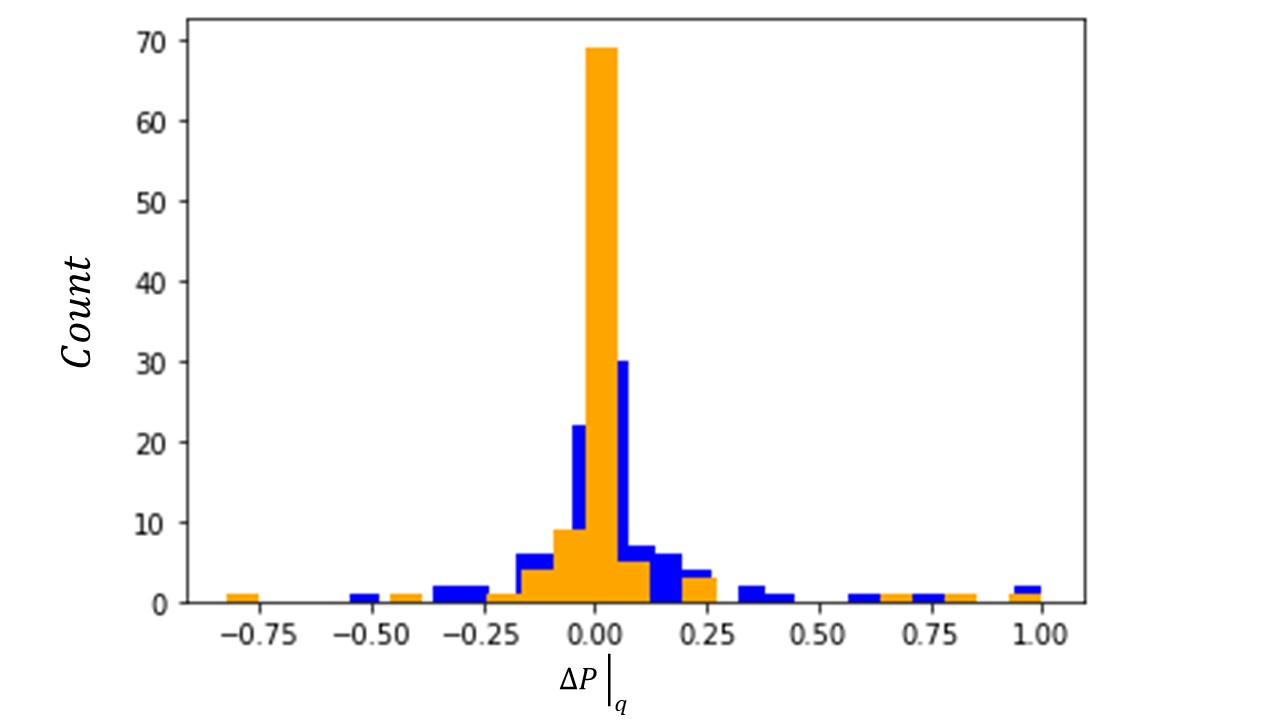
5. Results: Applying this repair method to the binarized Adult dataset, we find that 98 positive decisions were flipped in the female group, whilst 347 negative decisions were flipped in the female group. This suggests that the majority of the discrimination identified with this causal method was directed towards the female group. Below is a comparison of histograms for, calculated for each q, before (blue) and after (orange) the repair. This reveals the overall shift of the non-discrimination measures towards the center () following the repair, demonstrating the effectiveness of this debiasing tool. Moreover, the mean ofbefore the repair is 0.06, whereas, after the repair, the mean ofis 0.01, which suggests there is an overall reduction in female discrimination.

Conclusion

The detection and removal of bias with a causal approach has been investigated. We chose to take a more practical perspective so that this article could serve as a guide for practitioners going forward in this field. Firstly, we looked at different causal discovery methods, which are useful for identifying the causal structure of a dataset, and are often needed to perform a causal repair. Also, some open-source toolboxes related to causal discovery were outlined. Lastly, three causal repair methods from the literature were discussed, where one was implemented using the Adult dataset. According to the results from this implementation, the technique is successful in removing discrimination from the dataset, where the the mean of the discrimination measure, , decreases from 0.06 to 0.01 following repair. However, it is evident from the steps outlined, a considerable amount of background information is required before the algorithm can actually be imposed. This is a known issue with these types of repairs, which we previously discussed. As well, some of the results of the causal discovery toolbox were found to be inaccurate, such as the wrong direction of some arrows. Thus, although it is evident that they are useful tools for bias mitigation, the practicality of these forms of debiasing techniques is questionable. We believe that further research is needed in this space to develop algorithms that are easier to apply in practice. We hope this article does provide some guidance to practitioners and that it may inspire some more work in this area.

References

Chickering, D.M., 2003. Optimal structure identification with greedy search. The Journal of Machine Learning Research, 3: 507-554. https://doi.org/10.1162/153244303321897717

Colombo, D., Maathuis, M. H., Kalisch, M. and Richardson, T. S., 2012. Learning high-dimensional directed acyclic graphs with latent and selection variables. The Annals of Statistics, 40(1): 294-321.http://www.jstor.org/stable/41713636

Glymour, C., Zhang, K. and Spirtes, P., 2019. Review of Causal Discovery Methods Based on Graphical Models. Frontiers in Genetics, 10:1-15.https://www.frontiersin.org/article/10.3389/fgene.2019.00524

Salimi, B., Howe, B. and Suciu, D., 2020. Database Repair Meets Algorithmic Fairness. ACM SIGMOD Record, 49: 34-41. https://doi.org/10.1145/3422648.3422657

Spirtes, P., Glymour, C. and Scheines, R., 2001. Causation, Prediction, and Search,

2nd edn. Cambridge, MA: MIT Press.

Zhang, K., Peters, J., Janzing, D. and Scholkopf, B., 2011. Kernel-based conditional independence test and application in causal discovery. In Proceedings of the Twenty-Seventh Conference on Uncertainty in Artificial Intelligence (UAI'11). AUAI Press, Arlington, Virginia, USA, 804-813.https://dl.acm.org/doi/10.5555/3020548.3020641

Zhang, L., Wu, Y. and Wu, X., 2017a. A causal framework for discovering and removing direct and indirect discrimination, Proceedings of the Twenty-Sixth International Joint Conference on Artificial Intelligence, 3929-3935. https://doi.org/10.24963/ijcai.2017/549

Zhang, L., Wu, Y. and Wu, X., 2017b. Achieving Non-Discrimination in Data Release. In Proceedings of the 23rd ACM SIGKDD International Conference on Knowledge Discovery and Data Mining (KDD '17). Association for Computing Machinery, New York, NY, USA, 1335-1344. https://doi.org/10.1145/3097983.3098167

[a]Notebooks available in the ETIQ github repository:https://github.com/ETIQ-AI/ml-testing/tree/main/Causality%20Research